The Matrix Processor

The matrix processor is an example of a typical 'regular' problem.

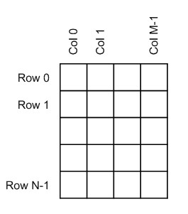
We require to compute a 2d Grid of values. All the elements from each Row are processed in a Row-by-Row calculation and similarly all elements from each Column are processed in a Column-by-Column calculation. Finally a result is computed from all of the Row and Column results. Each process is independent apart from the input data.

Sequential Solution

In the classic solution each result is calculated in turn.

while( TRUE )
{
   GridCell grid[N][M];
   RowCell rows[N];
   ColCell cols[N];

   // Populate the 2-D grid
   for ( int rowNum = 0; rowNum < N; rowNum++ )
   {
      for ( int colNum = 0; colNum < M; colNum++ )
      {
         CalcGrid( grid[rowNum][colNum] );
      }
   }

   // Do each row calculation
   for ( int rowNum = 0; rowNum < N; rowNum++ )
   {
      CalcRow( grid, rowNum, rows[rowNum] );
   }

   // Do each column calculation
   for ( int colNum = 0; colNum < M; colNum++ )
   {
      CalcCol( grid, colNum, cols[colNum] );
   }

   // Sequential output
   Output( rows, cols );
}

Parallel Solution

The sequential is fine on a single processor, however on a multi-core or multi-processor system this solution will only utilise a single core/processor. Parallelising this problem is not a trivial issue. Although it is clear that the NM Grid calculations, the N Row calculations and the M Col calculations can each be processed in parallel

while( TRUE )
{
   GridCell grid[N][M];
   RowCell rows[N];
   ColCell cols[M];

   // Populate the 2-D grid
   Parallel.For( 0, N, delegate(int rowNum)
   {
      Parallel.For( 0, M, delegate(int colNum)
      {
         CalcGrid( grid[rowNum][colNum] );
      } );
   } );

   // Do each row calculation
   Parallel.For( 0, N, delegate(int rowNum)
   {
      CalcRow( grid, rowNum, rows[rowNum] );
   } );

   // Do each column calculation
   Parallel.For( 0, M, delegate(int colNum)
   {
      CalcCol( grid, colNum, cols[colNum] );
   } );

   // Sequential output
   Output( rows, cols );
}

This is far from optimal. Each row calculation could start as soon as all of the elements in that row have been calculated, and the same is true for each column. Thus they can be executed in parallel with the Grid calculations. Similarly each Grid calculation can be restarted (for the next iteration) as soon as its Row and Col calculations have been done. In this way there is a potential NM + N + M +1 parallel jobs that could be performed. With double or higher buffering this could be pushed higher. Programming this using the current generation of 'parallel language extensions' is extremely cumbersome. The solution below parallelises the Row/Col and double buffers the Grid/Output calculations.

GridCell grid[N][M] = { 0 };
RowCell rows[N]    = { 0 };
ColCell cols[M]    = { 0 };

Action[] actionsGridOut = new Action[2];
Action[] actionsRowCol = new Action[2];

actionsGridOut[0] = delegate
{
    Output( rows, cols );
};

actionsGridOut[1] = delegate
{
   Parallel.For(0, n, delegate(int nn)
   {
      Parallel.For(0, m, delegate(int mm)
      {
         CalcGrid(grid, nn, mm);
      } );
   } );
};

actionsRowCol[0] = delegate
{
   Parallel.For(0, n, delegate(int nn)
   {
      CalcRow(grid, nn, rows[nn]);
   } );
};

actionsRowCol[1] = delegate
{
   Parallel.For(0, m, delegate(int mm)
   {
      CalcCol(grid, mm, cols[mm]);
   } );
};

while ( TRUE )
{
   Parallel.Invoke( actionsGridOut );
   Parallel.Invoke( actionsRowCol );
}

CDL Solution

The CDL circuit solution is shown below. This circuit uses a buffered pipeline/parallel structure, where each method is started as soon as its inputs are ready. With buffering set to 1 throughout, this circuit would behave like the 'Parallel code' above. However, increasing the Buffering allows the CalcGrid method to be restarted as soon as the associated Row/Col calculations have been completed (the same is true of the Col and Row calculations). This allows the maximum system concurrency to be extracted no matter what the architecture.

Click to enlarge

Uns CalcGridMthd::Process()
{
   // identify this cell
   Uns r= this->Element( 0 );
   Uns c= this->Element( 1 );

   // calculate cell
   return CalcGrid( r, c );
}

Uns CalcRowMthd::Process()
{
   // identify this cell
   Uns r = this->ElemNum();

   // calculate cell
   CalcRow( r );
}

Uns CalcColMthd::Process()
{
   // identify this cell
   Uns c = this->ElemNum();

   // calculate cell
   CalcCol( c );
}

Uns OutputMthd::Process()
{
   CalcOutput();
}

The CLIP documents 'Latent Task Concurrency' and 'Task Scheduling Latency' show theoretical and actual benchmarks for the CDL and parallel solutions for various N,M and task (CalcGrid, CalcCol etc) sizes.

The figures below show two examples of the application running, with different parameters.

Cells change colour each time their Method processes a data frame. The numbers show the current frame number being processed (black - in progress, white - finished waiting for next frame).

The Buffer Depth can be modified to increase the amount of run-ahead each method is allowed.

The Num Worker Threads controls the number of Methods that can be simultaneously active. This defaults to the Num of CPU cores.

The Load controls the size of the task that each Method performs. This can be randomized to generate a non-deterministic processor load balance. The load and randomization can be changed during execution.

The Matrix solution is available as a MSVisual Studio 2005 solution package from the Connective Logic Web site.

Blueprint Help	Send comments on this topic.
Matrix Processor